Overview

In the first project for CS184, I implemented a rasterizer which is capable of digitally drawing images, supersampling and antialiasing, transformations, and texture mapping through various methods. As a 3D Modeler and Animator, it was incredibly interesting to see the underlying process of how images are created, filtered, mapped, and rendered. Through this process, I've learned that even the most simple images take a great deal of effort to create, both artistically and computationally.

Section I: Rasterization

Part 1: Rasterizing single-color triangles

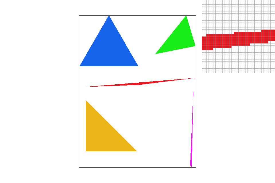
In the first part of the project, I built a triangle rasterizer which allows basic images to be digitally drawn. This process starts with the three vertices that define the edges or points of the triangle we are trying to rasterize. By looping through our image, pixel by pixel, we then want to determine which pixels in the image are "inside" our triangle. If a pixel lies within the bounds of our triangle, we want that pixel to be "rasterized" or filled in with the corresponding color. Though this made sense conceptually, I had a hard time understanding the computation behind this process as math was never my best subject. However, after a bit of reading and collaboration with classmates, I was able to get a better grasp of the situation. Another problem that arose in this process was understanding that if only given three points of a triangle, we cannot necessarily determine what direction, or how this triangle was drawn and that affected the outcome of the rasterization. In those cases, I'd sometimes get images that were only half filled since only half of the triangles were being rasterized. Once I accounted for both cases of directionality (i.e. whether the triangle was drawn clock-wise or counter clock-wise), the images were rendered sucessfully. However, another unforseen issue that I encountered was the runtime of the algorithim. Originally, my method was to loop through the ENTIRE image and test to see if each pixel was inside or outside the defined triangle. However, that meant that the runtime was unecessarily long, as it was oftentimes searching through blank or empty spaces of the image without reason. To fix this issue, I changed the bounding box of my looping method so that the algorithim would only search within the pixels defined by our three original points for each triangle. The result of this whole process were simple and beautiful rasterized images.

Part 2: Antialiasing triangles

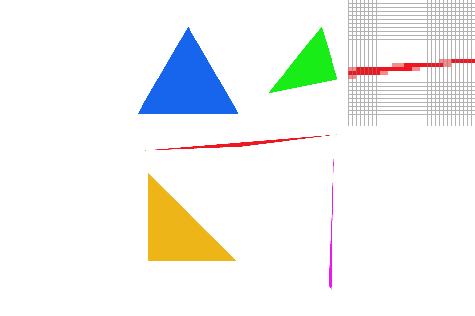
Part two of the project has us implement supersampling so that we can apply antialiasing to our images. Though the rasterization in part 1 is successful, there are clear examples of 'aliasing' in the images. In other words, they seem pixelated and "jaggy" around the edges of the triangles. To fix this problem, we want to sample the image at a larger rate. A larger sample size gives us more information about each pixel by computing sub pixel values. With this, we can find the average color around the edge of the triangle and implement a gradient value, rather than a solid, harsh line that cuts off at each pixel. This gradient helps give the illusion and a cleaner image and reducing the "jaggies" for every rasterized triangle. As a result, supersampling functions as an efficient method of anti-aliasing. The algorithim was very similar to the one I wrote in part 1, however, I needed to add another set of looping functions that could find the sub-pixel for each pixel as well as a function to find the average color for the sub-pixels.

Part 3: Transforms

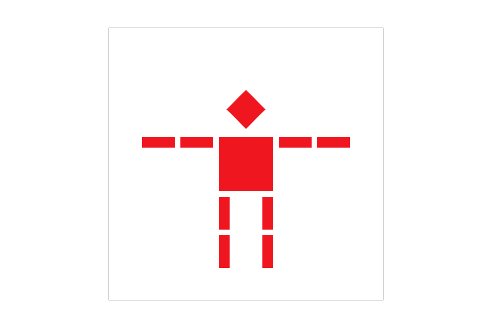
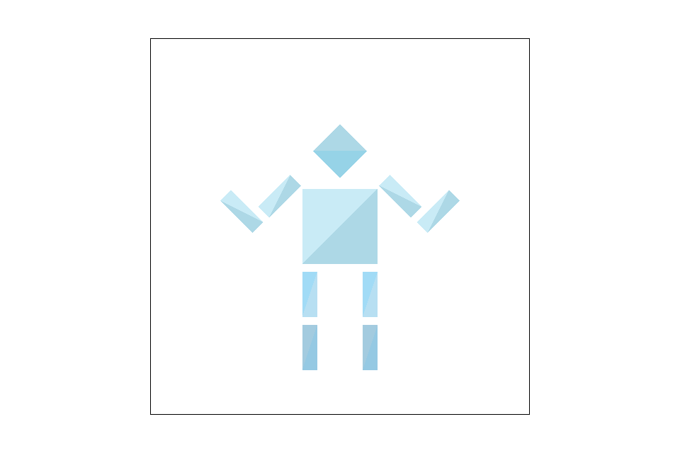
Part three of the project was probably my favorite for two reasons: it was the part I understood best conceptually and it allowed us to create something personal and fun in the process. The goal of this section was to implement basic transformations such as translation, rotation, and scaling to 2D images. These transformations can all be represented as a system of linear equations, which means that we can simplify this process as a series of matrix operations With some simple linear algebra, we are able to turn some oridinary squares into a lively little robot! (Or a confused one)

Section II: Sampling

Part 4: Barycentric coordinates

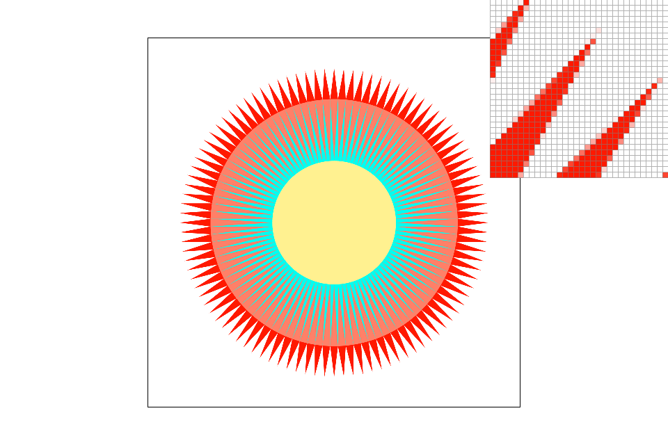
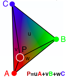
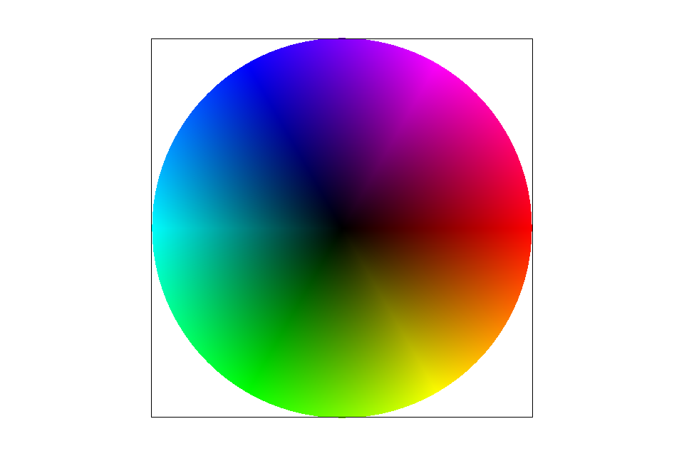
In part four of the project we implemented the calculation and usage of Barycentric Coordinates. Barycentric coordinates allow us to find the location of any point (x,y) inside of our rasterized triangle which can be useful for returning colors at a specific location and texture mapping which we will talk about in the next steps. Calculating these coordinates is relatively simple (even for someone who is as elementary in math as I am). Essentially, we need to find the lines that represent the distance between each vertex of the triangle (A, B, C) and the point P we are trying to find. These line equations are represent our "alpha", "beta", and "gamma" values that will be multiplied to the color at each edge vertex. In the end, these coordinates are immensely helpful in the next few steps of the project as well as in graphics in general. They help turn an ordinary, black circle into a wonderful color wheel complete with gradients.

Part 5: "Pixel sampling" for texture mapping

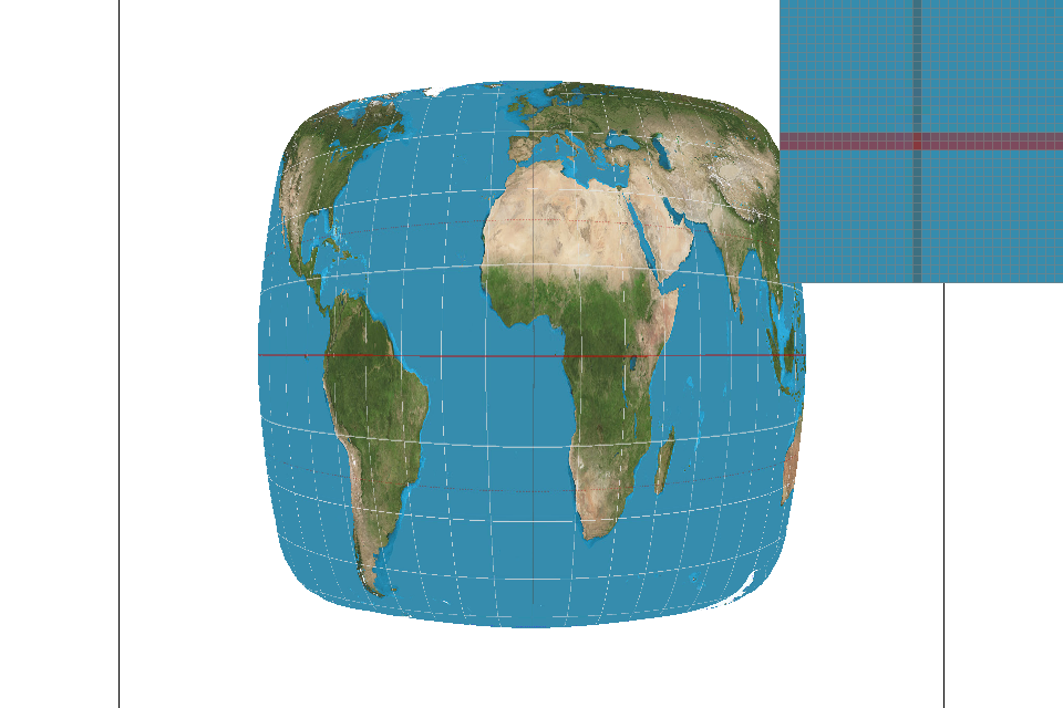
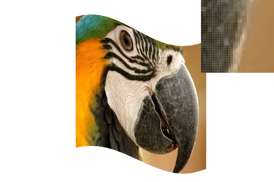
Eariler in the project, we practiced sampling with the implementation of super-sampling. In part 5 we repeated a similar process with texture mapping! Essentially, we have pixels in our screen space (x, y) that correspond to points in our texture points (u, v). Therefore the process we had to follow to implement texture mapping was similar to sampling or re-sampling. We had to first iterate through our pixels in the screen space, find the corresponding u, v coordinates in the texture space with the use of Barycentric coordinates from the previous section, and finally use these coordinates to perform the desired sampling method. In our case, there were two sampling methods that mapped the textures and provided slightly different results in terms of aliasing. First, there is nearest sampling, in which we determine the surrounding pixels that are closest to our u,v coordinate and return the texture color (texel) of the pixel with the minimum distance. Then there is bilinear sampling; this method alternatively finds the texel values of the pixels surrounding our u,v coordinate and then interpolates between these values. So, rather than returning one texel value, we are returning a combination of several pixels. These methods can lead to drastically different results when it comes to anti-aliasing. In the images below we can see that bi-linear sampling results in less noise in the image. For instance with the texture of the globe, there are random areas of noise in the image rendered with nearest sampling. The line of the equator is similarly mis-drawn and results in the image looking a bit noisy. In comparsion the image rendered wit bi-linear sampling has a cleaner line at the equator and less noise in the texture. A similar shows with the textures of the parrot. Bi-linear sampling allows for a smoother gradient of the texels and results in less "jaggies" in the image. These differences seem trivial in concept but in practice they make a big difference.

Part 6: "Level sampling" with mipmaps for texture mapping

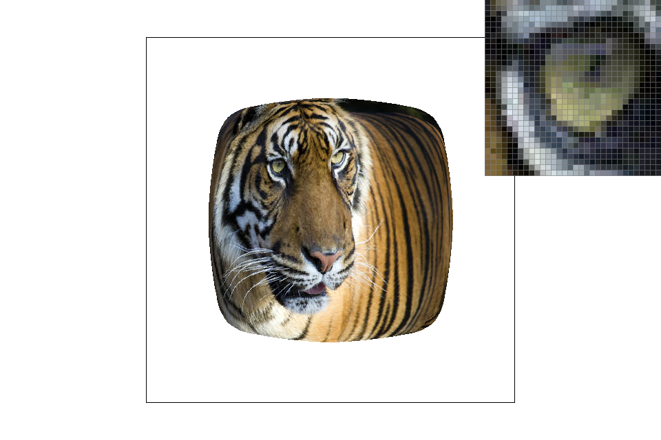
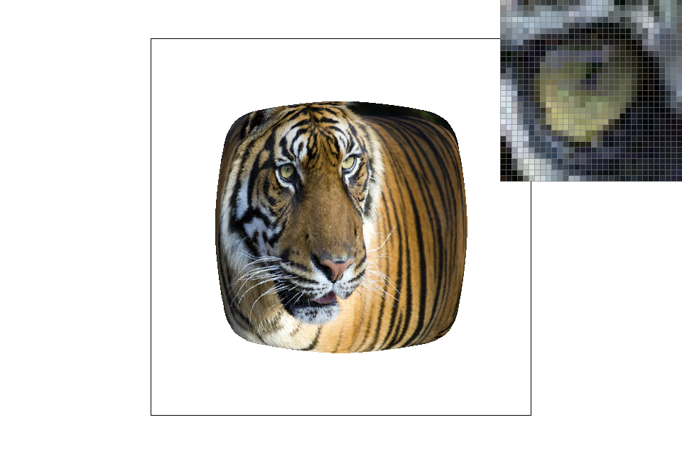
In the final section of the project, we further developed our rasterizer's capability of texture mapping by accounting for level sampling. In addition to sampling at different methods, we can also sample at different levels. In doing so, we are accounting for the level of resolution that we are sampling at, and utilize this mipmap level to filter our image. This can result in an image with drastically reduced aliasing. To implement level sampling, we had to first write a method that could successfully find the level of sampling we were using. Then, we would pass that calculated level into our sampling methods from the previous section, except this time they are accounting for the level of mipmap being used. In the end, we see the difference in the images. Each combination of level sampling and sampling method produced a texture map with varying amounts of aliasing with the most clear being tri-linear sampling (linear leveling and linear sampling) being the most anti-aliased. However, each method does come with its own share of rendering and calculation costs. For example, certain images, if they are too high-resolution, will not tri-linearly sample as it is double cost of bi-linear sampling. In this case, you are trading rendering speed and memory usage for better antialiasing. In the case of sampling at level zero and using the nearest sampling method,our trade offs would be converse. At the end, the results speak for themselves, and it depends on the artist and creator which method suits them best. Sometimes efficency and speed can lead to beautiful works alone (VR games being a prime example) so it's naive to say that any one method is supreme than the other in the same ways. No matter what method of sampling you choose, the end result is always satisfying to see.