Assignment 3-1: PathTracer
Ashna Choudhury
In project 3-1 of CS184, we implemented elements of pathtracing and raytracing which included various lighting simulations such as direct, indirect, and global illumination. Combined with different sampling methods to optmize the process resulted in images that were more efficently rendered as well as outputted with less noise. This project dealt mostly with diffuse materials and simulations though in future projects we may explore more reflective materials and their effects on rendering. Throughout my years in college I've been familar with the process of rendering, as well as the many hours it takes to complete, however after completing this project I certainly have a greater appreciation for the underlying computations, equations, and especially the beautiful final images that take so much time to create.
Part 1: Ray Generation and Intersection
In the first part of the project, we implemented the first steps of pathtracing that make rendering possible. This incredible process starts with the idea of generating rays from the camera or the eye to various parts of the scene. To do this we began with a simple loop that ran to an equivalent number of samples we wanted to test per pixel. For every sample in this pixel, we created a new ray from our camera and projected it into the scene. Once a ray is created, we need to test if it will intersect with any of the objects inside of the scene. If it does then we want to draw or render that triangle or primitive it intersected.
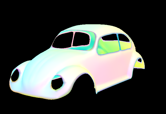
As we did in project 1, we began with the most commonly used intersection test which was for triangle based primivites. In this assignment, we used the Moller-Trumbore algorithim to determine the time of intersections (if they exist) as well as the bary-centric coordinates that will be needed to render the normals of the triangle. Math has never been my best subject so implementing this equation was admittedly difficult for me, but after several hours of attempts, the final results are certainly worth it. With ray generation and triangle intersections implemented properly we are able to render a simple (but elegant) image below.
 Result of generating rays and testing for triangle intersections
|
After implementing sphere interesection tests utilizing the quadratic formula we are also able to render images with sphere primitives in them.
 Generating rays and testing for sphere intersections
|
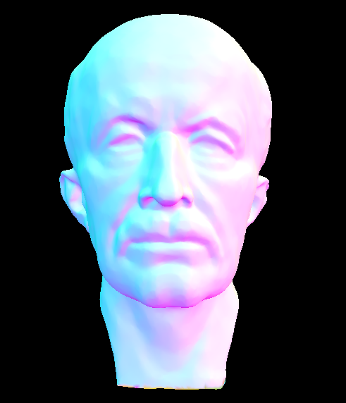
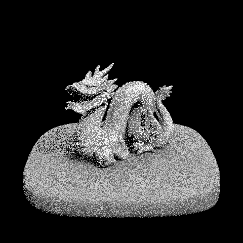
 Meet Lucy
|
Part 2: Bounding Volume Heirarchy
Though the images in the previous part were beautiful, they were relatively simple, and unfortunately, rendering anything more complex at that point would take a very long time or simply crash upon execution. Thankfully, in part 2 of the project we implemented bounding volume heirarchy in order to optimize our calculations and rendering time. In theory, this process is a way of "dividing or splitting" our primitives into smaller and smaller boxes and test for intersections to those bounding boxes rather than the whole scene. If a ray does not hit a bounding box, then we know that it does not hit any of the objects inside of it, and therefore we can skip the process of testing intersections with that area of the scene.
This process starts with constructing the Bounding Volume Heirarchy which is represeted as a binary tree in our code. However what is most important about this whole process is the way in which we pick our "split points" or essentially how we divide the objects into these bounding boxes. For this implementation, my split point was calculated based on the average point between all the primitives' center points or centroids. Then, for each axis, we want to check whether each primitives' centroid is less than or greater than this split point. If it was less, then we sorted that primivtive into the left branch, and if it was greater than it placed in the right branch. When recursively called, this process successfully splits our mesh into a bounding volume heirarchy.
Now that we have this heirarchy, we can simply recurse through our tree bottom-up. Essentially, we check if we are at a leaf node, if not, then we want to recursively call this method until we reach the leaf nodes. Once we are there, we can loop through all of the primitives at that level and test for intersections using the methods we wrote in the previous.
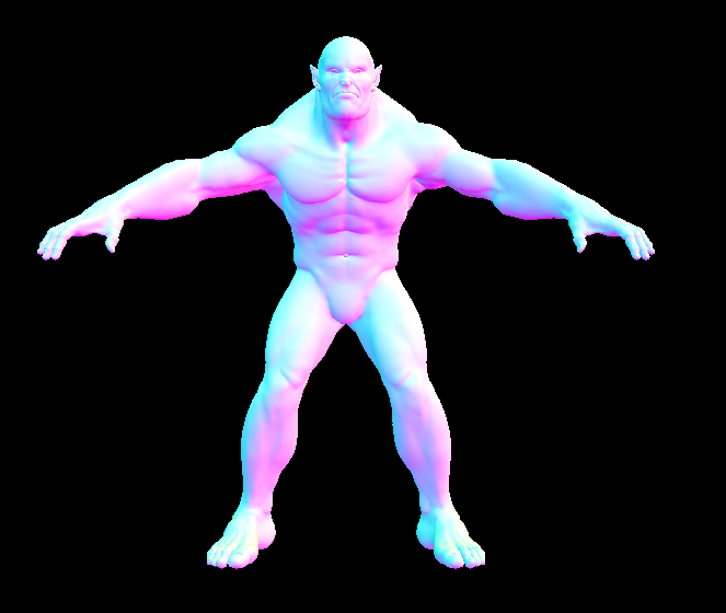
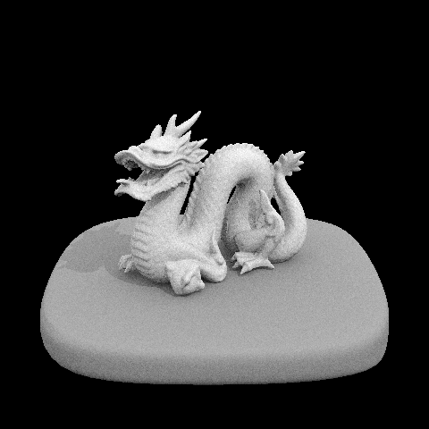
The end result is a much improved render time for heavier meshes. We are now able to render high poly files (which should look familar from the last project) in a matter of seconds.
The render time for the cow image, for example, improved from 3 minutes to 3 seconds. This optimization makes rendering the more complicated images in later parts possible.
Part 3: Direct Illumination
In part 3 of the project, we implemented two methods of direct lighting: uniform hemisphere sampling and importance sampling.
Uniform Hemisphere Sampling
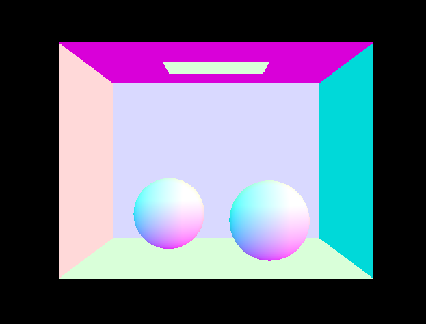
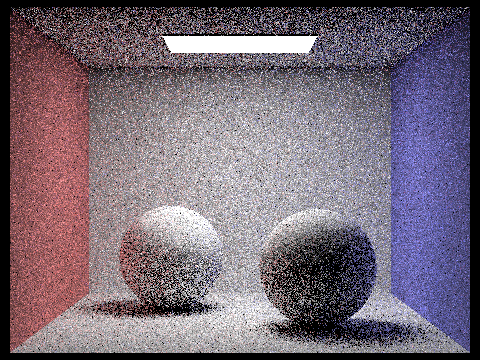
In hemisphere sampling, we simulate light uniformly in the scene rather than evaluating each light in the scene differently. As a part of this, the probability density function or PDF used in evaluating light in the scene does not change and is kept at a constant of (1/(2 * PI)). First, we want to represent the rays that are coming into the scene. Then, using methods written in previous parts, we want to check if this ray intersects with the current hit point we are evaluating. If it does intersect, then we want to calculate the irradiance at this intersection and sum it to our final spectrum value that represents the light coming from this point. The result successfully renders a uniformly sampled scene as we can see from the image of lambertian spheres below.
 CBSpheres Uniform Sampling: 16 Samples, 8 Rays
|
Unfortunately, even if we were to sample at a higher rate, the image does contain a lot of noise. The next method of sampling, however, improves upon this noise!
Importance Sampling
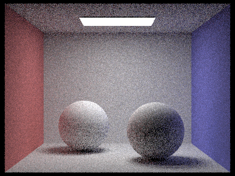
Importance sampling, in comparison to uniform hemisphere sampling, takes samples from each light source and accounts for this into its final evaluation of the scene, giving way to more defined renders. Therefore, the biggest difference in implementation for this part was to first loop through each light source in the scene before creating rays or calculating radiance. Once we take samples from our current light source, we can continue to generate rays, test for intersections, and sum our spectrum values. In the end, we can see the final image has much less noise!
 CBSpheres Importance Sampling: 16 Samples, 8 Rays
|
Since importance sampling is based upon sampling from the light sources, changing the number of light rays in the scene has a heavy affect on the final renders. As we can see in the images below, when there is only one light ray, the image becomes quite noisy and blurry. However, with each increase of light rays, the image becomes clearer and clearer. This is slightly from uniform sampling in which the number of samples has a much bigger effect on the final result.
 1 sample & 1 light ray
|
 1 sample & 4 light rays
|
 1 sample & 16 light rays
|
 1 sample & 64 light rays
|
 64 samples & 32 light rays produces impressive results!
|
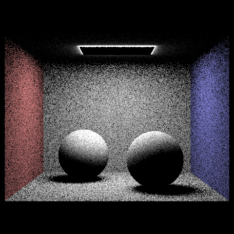
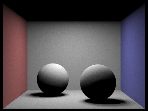
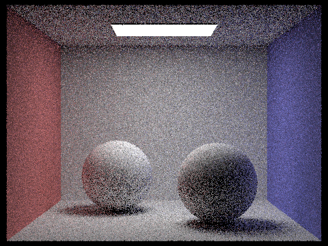
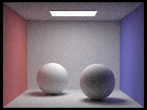
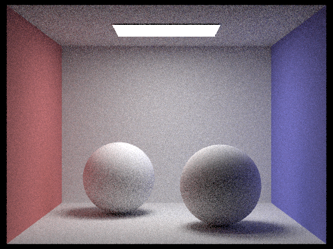
In the end, importance sampling produces significantly less noisy images than uniform sampling. As we can in the images below, even though we are sampling at 64 pixels, the uniformly sampled image is still grainy and unclear while the other image is much cleaner. To get an equal high-quality image from uniform hemisphere sampling, we would have to increase the samples per pixel much more. This is potentially less efficient and more costly on render time than it would be to add a few more light rays into the scene for importance sampling.
 Uniform Sampling: 64 samples & 32 light rays
| | | | |
|
 Importance Sampling: 64 samples & 32 light rays
|
Part 4: Global Illumination
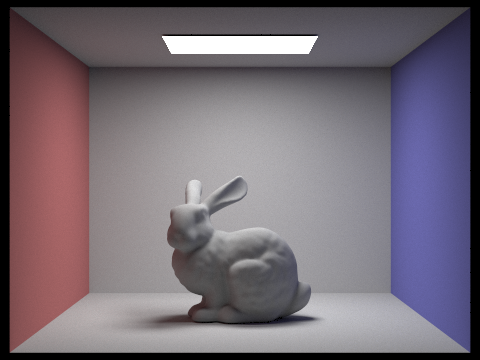
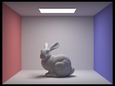
In this part of the project we implemented global illumination which is calculated by summing the direct and indirect lighting of the scene. Direct lighting was implemented previously in part 3 and corresponds to either uniform hemisphere sampling or importance sampling. Therefore in this part, the main functionality was to implement indirect lighting, and then take the sum of zero bounces in the scene, one bounce into the scene (direct lighting) and all other bounces in the scene (indirect lighting). Since indirect lighting can continously bounce around the scene, we want to implement this function recursively, with each recursive call summing to the final output. However, one important condition to add in this process to make sure that we don't bounce rays infinitely, is to add a termination probability. This termination condition is based on the "Russian Roulette" theory which basically picks a very small random probability to terminate this process on. After successfully recursing, summing, and scaling our final output, we can take this total sum as our global illumination of the scene. As we can see in the images below, the simulated light is much more complex and takes the indirect bounces of light from the walls and light sources into account.
 CB Bunny - Global Illumination
|
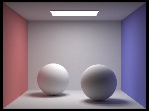 CB Spheres - Global Illumination
|
We can break down this idea of summing our global light by separating our direct and indirect illumination of the scene. The image on the left is the result of the direct lighting (uniform or hemisphere) that we calculated in the previous part, while the image on the right is the result of the indirect lighting we calculated in this section. Therefore when you take the sum of the two lighting evaluations, you get the final global illumination of the scene.
 Only Direct Lighting
|
 Only Indirect Lighting
|
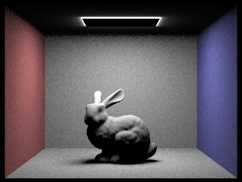
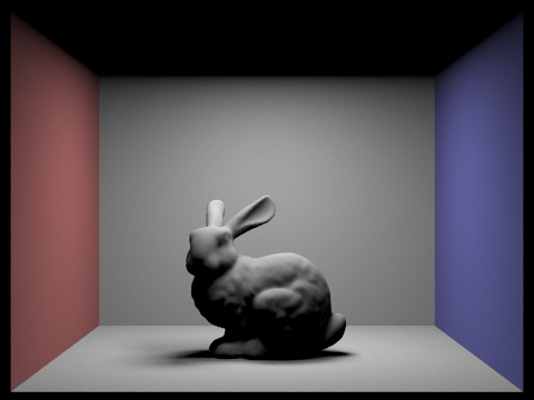
Changing the max ray depth, or the maximum depth of bounces for each ray, changes the output of the image. If we set our max ray depth to zero, then this is equivalent to no light bounces in the scene which will only result in the light source in the scene being shown. If we change this value to one, then the ray is allowed one bounce in the scene and results in direct lighting. When max ray depth is greater than or equal to two, we start to see the effects of indirect lighting, with each increase making the render slightly brighter than before. For example, at 100 max ray depth, the image is the most bright which can be seen in comparing the shadows in the back wall and on the floor.
 Max Ray Depth = 0, Samples = 1024
|
 Max Ray Depth = 1, Samples = 1024
|
 iMax Ray Depth = 2, Samples = 1024
|
 Max Ray Depth = 3, Samples = 1024
|
 Max Ray Depth = 100, Samples = 1024
|
Changing the number of samples per pixel also affects the final render. Lowering the sample number results in more noise while increasing the sample number leads to clearer results.
 1 Sample, 4 Light Rays
|
 2 Samples, 4 Light Rays
|
 4 Samples, 4 Light Rays
|
 8 Samples, 4 Light Rays
|
 16 Samples, 4 Light Rays
|
 64 Samples, 4 Light Rays
|
 1024 Samples, 4 Light Rays
|
Part 5: Adaptive Sampling
In the last part of the project we implemented adaptive sampling, which selectively samples the image based on which areas of the scene are more complex and therefore need more samples. This means going back to the beginning of the project in which we implemented ray generation and intersection tests. Going to the original loop we created to iterate through the pixels and rays of the image, we want to test whether certain pixels have converged. To do this, we simply need to keep track of a pixel's mean and standard deviation with every sample we take. After successfully implementing adaptive sampling, our renders can deal with noise in a image without having to uniformly process the entire image. Therefore it is both efficient and helpful for final renders. We can see what areas of the image are "more complex" or importance based on the rate image on the right. It serves almost as a heat map of the render with red and green areas needing more attention than blue ones.
 CB Bunny 1024 Samples - Adaptive Sampling
| | | | | |
|
 CB Bunny Sampling Rate Image
|
After all of this hard work we are able to successfully render diffuse images!