CS 184 | Pathtracer 2

In Project 3-2, our goal was to push the functionality of our pathtracer from the previous project to handle rendering cases such as material modeling, environment lighting, and camera affects such as depth of field. With these new implementations, our pathtracer can successfully render different materials like glass, mirrors, and microfacets, process outdoor lighting simulations, and render through complex cameras.

Similar to previous projects, there were many hours of debugging, rendering, writing, and coding to produce these images, and the entire process certainly teaches one to be grateful and proud of the work it takes to create art.

Part 1: Mirror and Glass Materials

In part 1 of the project, we built upon the work that was done in project 3-1 such that our renderer can now process materials beyond diffuse ones. In this case, our goal was to simulate glass and mirror materials, which required calculating the BSDF for said materials as well as the implementation of reflections and refractions. As with most aspects of this project, the magic of the simulation comes from a basis in math and sometimes physics such as the following equation for reflection:

Here wi & wo refer to the input and output vectors that hit the material and bounce off of it.

*wi = -wo + 2*(dot(wo, n)) * n;

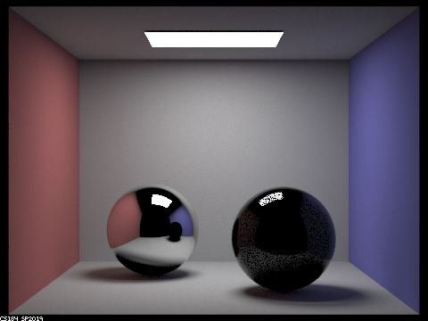
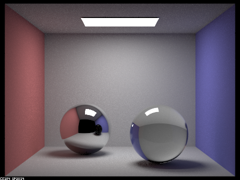
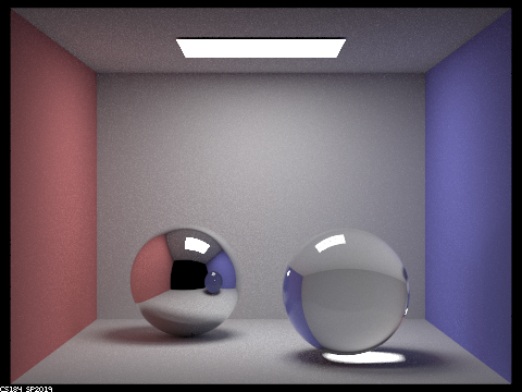
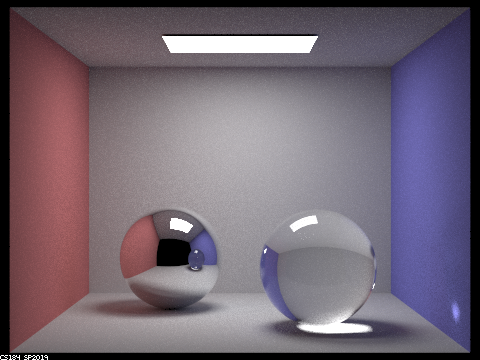
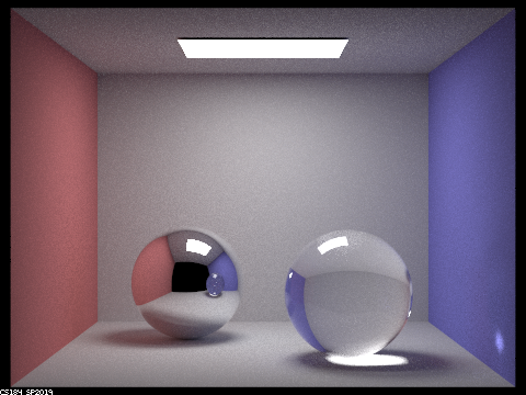
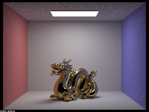
As we saw in the previous project, rendering with global illumination and varying ray depths in the scene result in different images. However, this time we can see that the surface of the spheres are drastically affected as well due to their mirror and glass-like materials.

In the first image on the top left we are rendering with a max ray depth of zero which is the equivalent of only evaluating the light coming directly from the light source and NO other light bounces in the scene, therefore the render is almost completely dark. In the second image with a max ray depth of one, this is the equivalent to rendering with direct lighting only, therefore the indirect bounces of light are not calculated. As a result, the room is much darker and the spheres are completely black as both mirror and glass material require more than one bounce of light to simulate the material. When we increase the max ray depth to two, the mirror material starts to exhibit more normal behavior although it is still quite dark, however the glass sphere still cannot render properly until there are three or more bounces of light in the scene. This is because the glass material needs light to travel through it rather than just hit the surface compared to the mirror material. As the bounces of light continue to increase we see that the renders are able to simulate more and more intricate lighting effects such as the circle of light reflected on the floor at m = 4 and the bounce of light against the right purple wall at m = 5.

Max Ray Depth = 0

Max Ray Depth = 1

Max Ray Depth = 2

Max Ray Depth = 3

Max Ray Depth = 4

Max Ray Depth = 5

Max Ray Depth = 100

Part 2: Microfacet Materials

In part 2 of the project we furthered our implementation of material modeling by simulating microfacet surfaces. This includes materials like copper, gold, aluminum, silver etc. The core of these simulations come from the following equation to evaluate the BRDF for Microfacet Materials.

Here, the fresnel term, shadow masking term, and normal distribution function (NDF) are all functions we implemented for the final result.

f_val = (fresnel_term * shadow_mask_term * NDF)/(4 * (dot(n, wo)) * (dot(n, wi)));

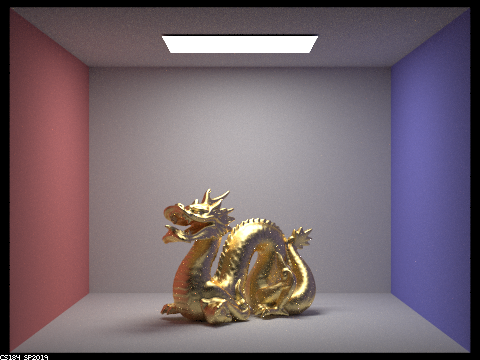
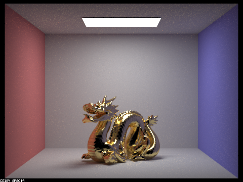
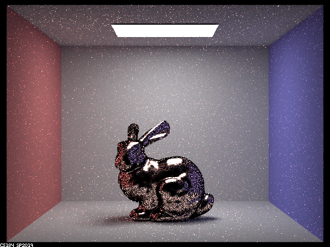
Each value in the above equation has an affect on the final render. The NDF, for example, defines the distribution of normals on the microfacet surface and one of the most notable values in its equation is the alpha value. The alpha value effects how diffuse or shiny the material will be. In the images below, we can see that when the alpha value is larger at 0.5, the final result is more diffuse and rough. As the alpha values decrease, the dragon becomes more shiny and glossy, giving a different kind of gold material.

Alpha = 0.5

Alpha = 0.25

Alpha = 0.05

Alpha = 0.005

As in the previous project, here we implemented two types of sampling: hemisphere sampling and importance sampling, and once again, we can see a notable difference in noise. The image on the bottom left utilized hemisphere sampling and has noticeably more noise than the image on the right that used importance sampling. Specifically in brighter areas of the image such as the hightlights on the bunny, we can see that importance sampling is able to render those highlights smoothly in comparison to the speckled image on the left. Importance sampling is also able to better handle the materials' golden or silver color around the edges of the bunny while in hemisphere sampling those edges are rendered much darker than they should be.

Hemisphere Sampling, Samples = 64

Importance Sampling, Samples = 64

After successfully implementing all of these functions, we are able to simulate many microfacet materials even beyond the ones initially given in the tests. For example, by looking up the spectrum values at specific wavelengths for a material like titanium, we are able to make a few minor changes and render a titanium bunny instead of a copper one.

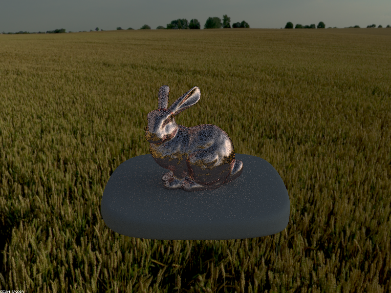
"Shoot me down...I won't fall... I am TITANIUM!"

Part 3: Environment Lighting

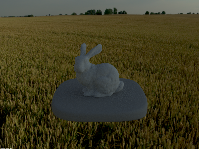
In part 3 of the project we stepped into new territory in terms of lighting and implemented environment lighting. In contrast to the lighting setups we have been using up until this point, environment lighting lights a scene from ALL directions at a distance that is no longer fixed to a specfic light source that can be seen in the setup. In other words, the light comes from many sources that are infinitely far awawy rather than specified lights that are fixed in the scene at a finite distance. Though it can also be used for indoor lighting, environment lighting is meant to simulate the sun and its affect on objects in an outdoor setting. As a result, many artists use environment lighting to give realistic simulations of outdoor lighting in day or night. For example, in the next few renders, the following .exr image below of an open field and the sun shining on it was used to simulate environment lighting.

The .exr map I used for Environment Lighting

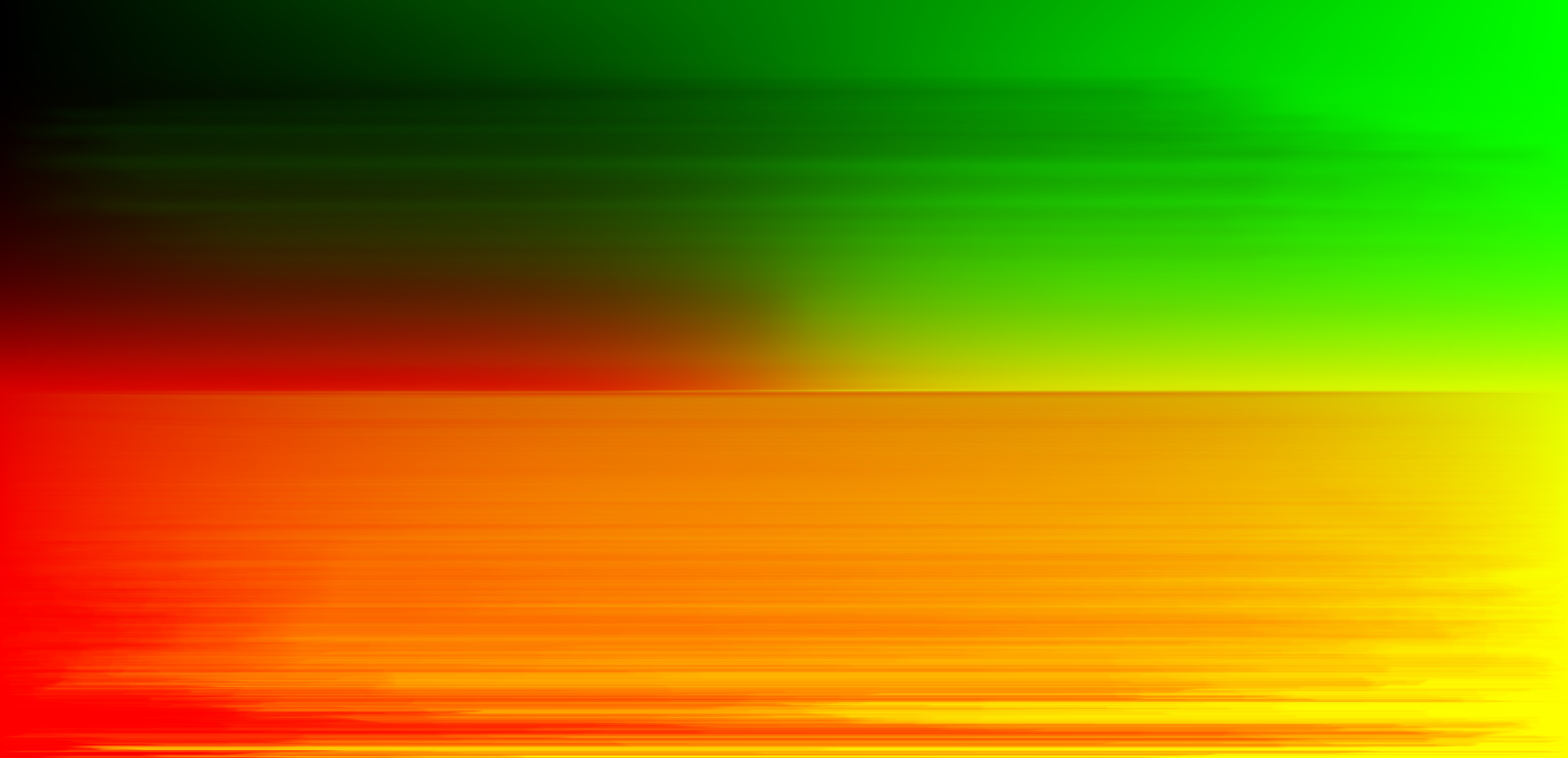
We implemented both hemisphere and importance sampling for environment lighting to see the different results. With importance sampling, we need to know which areas of the environment map give off more radiance. The image below is a map of the probability output for each pixel in the environment map. It serves as a way of debugging and discerning which parts of the map, give off how much intensity to the render.

The probability output image from this environment map

In the following examples, the difference between hemisphere sampling and importance sampling is much less drastic compared to previous implementations. However there are still changes in noise and brightness of the final renders. In the top left image that utilized hemisphere sampling, for example, we see that bunny is much darker compared to the image on the top right which used importance sampling. The details on the bunny's back and face are more blurred out in the hemisphere image compared to the importance image, and we can see more noise in lighter areas such as the bunny's back, left side of the face, and the pedestal.

We can see more differences between hemisphere and importance sampling in the bottom images of the copper bunny. Similar to top images, the image that was importance sampled is both brighter and has less noise in brighter areas of the render. If you compare the highlights on the bunny's back, ears, left half of the face, and on the pedestal, you will see less noise and speckles in the render on the right.

Hemisphere Sampling Unlit Bunny

Importance Sampling Unlit Bunny

Hemisphere Sampling Copper Bunny

Importance Sampling Copper Bunny

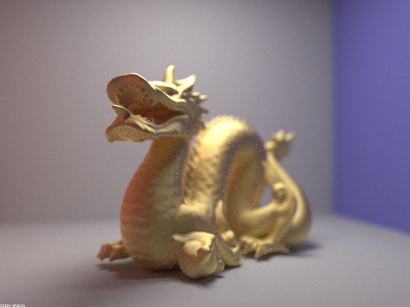
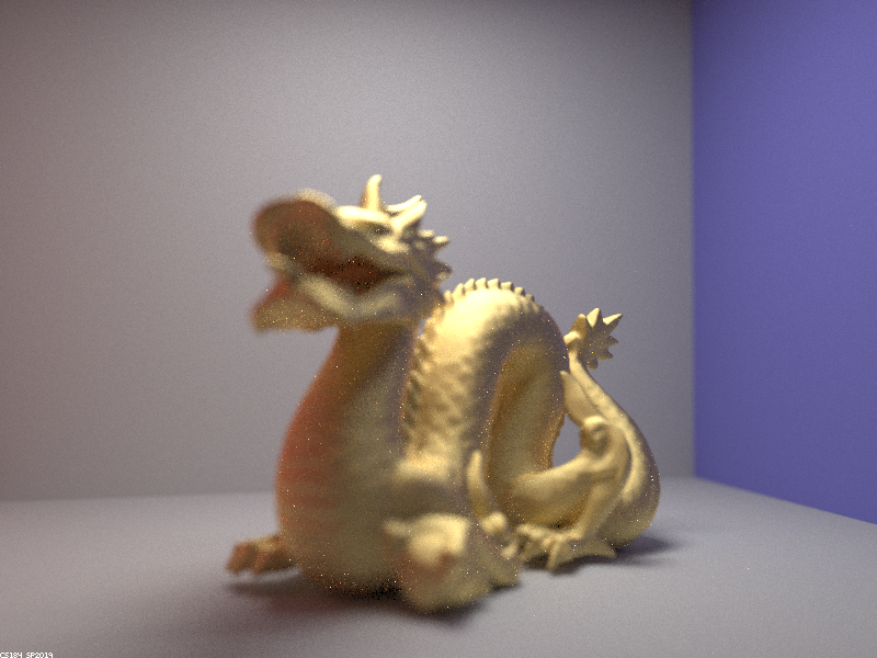
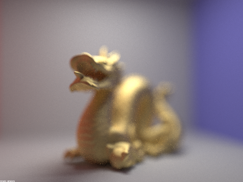
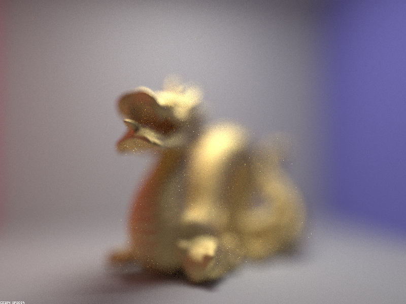
Part 4: Depth of Field

In all previous parts of this project as well as throughout project 3-1 we always rendered our images using a pin-hole camera. In this part, we implemented and utilized a thins lens camera which produces drastically different results. A pin-hole camera is a camera that renders/captures everything in focus. Notice in all of our previous renders the entire image was clearly visible. However, real cameras in film and and in life often don't capture the whole image in focus, but rather blur out parts of the scene to give a sense of depth. This would be created by the thin-lens camera, in which the ray traced from the image plane to the focus plane is refracted by the camera lens, in comparison to pin-hole camera ray which travels straight from the image plane to the focus plane.

Once we have implemented this thin-lens camera model, we can simulate very complex camera effects in our renders such as depth of field. In the following images, we can see the same dragon taken from the same angle but with different focal distances. This results in different areas of the dragon to be in focus, while other areas are blurred, and gives way to some wonderful opportunities for creativity.