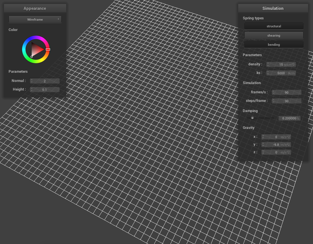
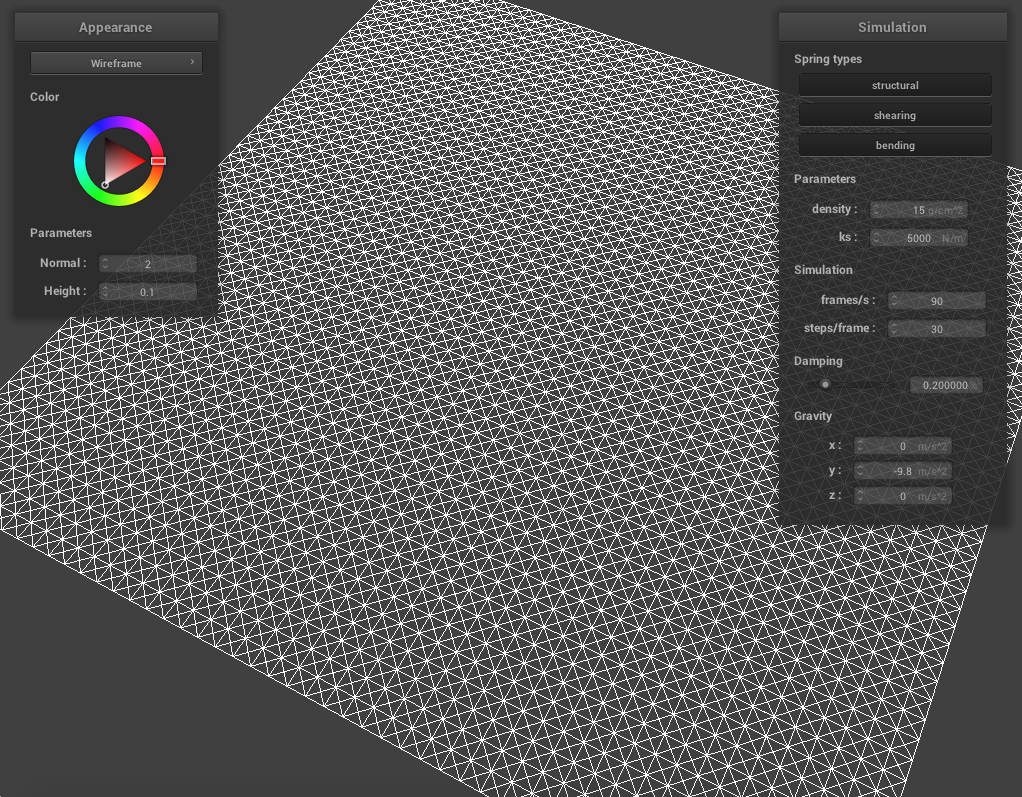
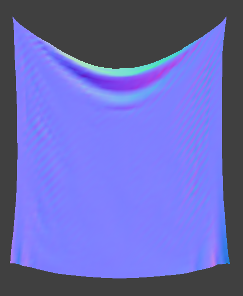
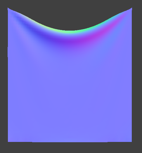
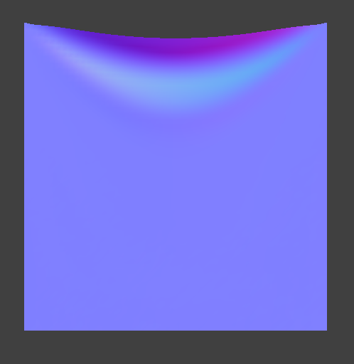
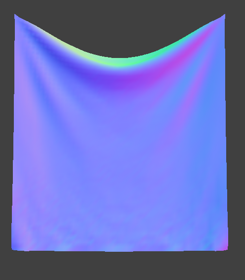
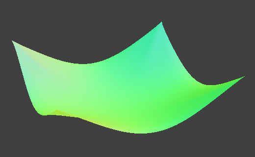
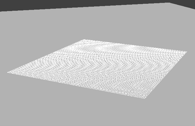
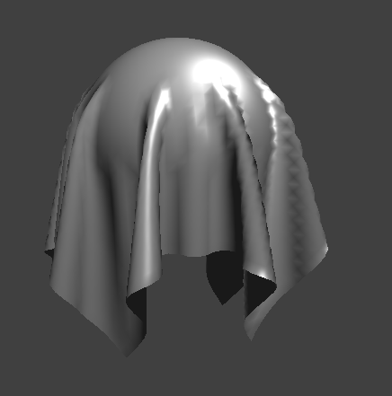
Before we are able to implement any elements of a cloth simulator, we will need to build the system of springs and masses that represent our cloth. First, we built our masses with a simple double for loop through our grid and creating the proper offsets for the x,y or z coordinates depending on horizontal or vertical orientation. Along the way, we needed to account for the point masses in our grid that would be "pinned" so that our cloth can hang properly in the simulation. Next came the springs and since there are different types of springs that can be used in the simulator, we had to account for the construction of each of these spring types which included structural, shearing, and bending constraints. After several rounds of careful checking and picky edge cases, we finally have our finished grid of point masses and springs which become heavily utilized in the rest of the project. For example, we can now isolate which types of constraints we want to use in our simulation. In the images below we see the different results of having a grid with no shearing constraints, with only shear constraints, and with all three constraint types.
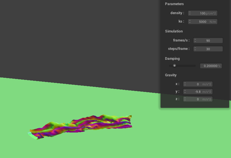
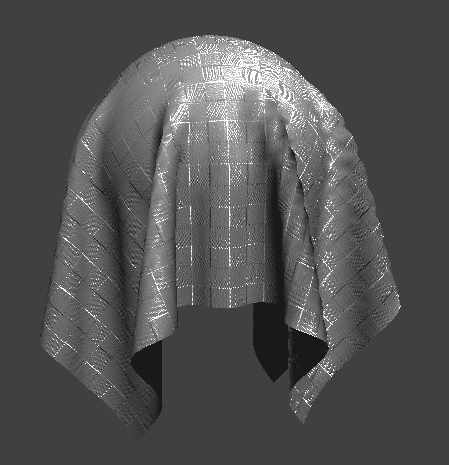
 No Shear Constraint
|
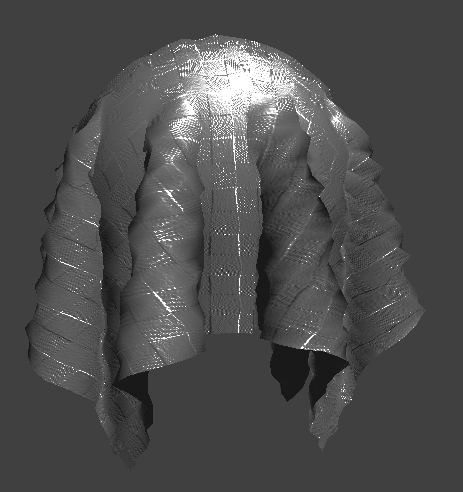
 Only Shear Constraint
|
 All Constraints
|
Part II: Simulation with Numerical Integration
In part 2 of the project, we began the actual implementation of simulating the cloth. This starts with computing the total external force that is acted upon all of the point masses on the grid. Next, we have to add on the unique forces being acted upon the springs which takes into account the type of spring constraint we are using. For example, while structural and shearing constraints have similar force vectors acting on them, bending constraints take are scaled by additional float value in the calculations. Once we have these force vectors we can apply them in equal but opposite strengths to two point masses for each spring. Our next step is to update the positions of each point mass using Verlet Integration which is described by the following equation.
x(t+dt) =xt + (1−d) * (xt − xt−dt) + at*dt^2;
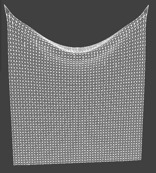
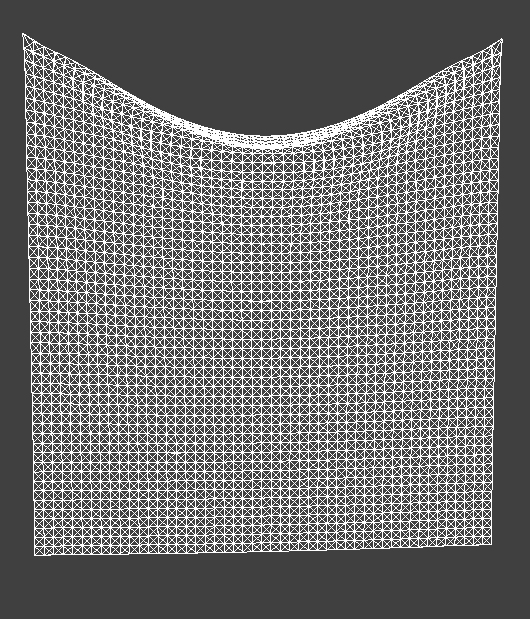
Once we've implemented these two steps the majority of our simulation is actually complete! However, there are some areas of the cloth that stretch more than they should, so to account for that we have to further modify the positions of each spring's point masses so that they are not too far apart. The difference between the cloth before and after this modification can be seen clearly in wireframe, especially near the corners.
 Before Additional Constraints
|
 After Additional Constraints
|
With these steps completed, we now have a functional cloth simulation!
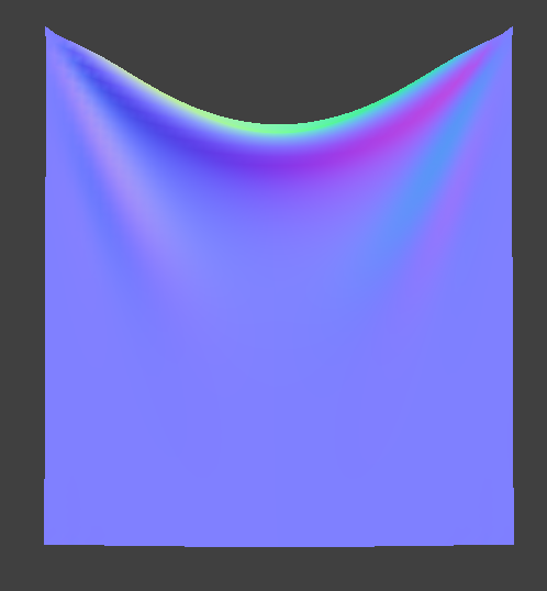 Simulation with Default Parameters
|
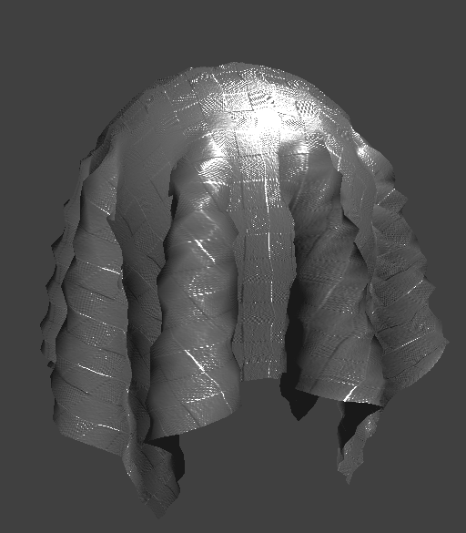
The output of the simulation can be changed by varying parameter values such as ks (spring constant), density, and damping which affects different attributes of the simulation and allows us to simulate different kinds of cloth. For example, when ks seems to have an affect on the firmness and/or thickness of the cloth: when it is set to a low value of 100 N/m, the cloth appears thinner and has more wrinkles running down the middle. As the simulation starts, the entire cloth sags limply and various lines run through the cloth until it stabilizes. In comparison, when ks is set to a higher value of 8000 N/m, the simulation starts with the cloth firmly falling without sagging far, and by the end, there are only a few major wrinkles in the mesh giving the feeling of a thicker, more durable cloth.
 ks = 100 N/m
|
 ks = 8000 N/m
|
On a similar note, density, seems to effect the bending strength of the cloth as when the density is low at 1 g/cm^2, the cloth sticks in place without much deformation. On the other hand, when the density is much higher at 100 g/cm^2, we see it bend much further.
 Density = 1 g/cm^2
|
 Density = 100 g/cm^2
|
Finally, damping also gives way to more or less wrinkles on the cloth as we see that decreasing damping results in more folds while increasing it will cause less/fewer defined wrinkles.
 Damping = 0.08 %
|
 Damping = 0.8 %
|
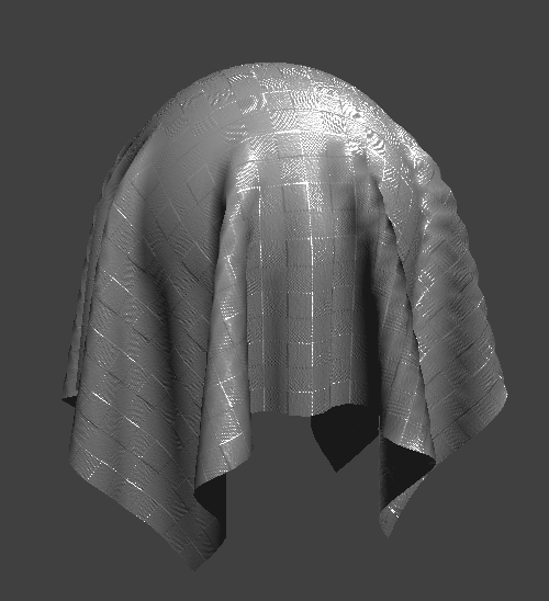
 4 Pinned Corners with Default Parameters
|
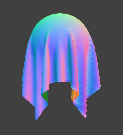
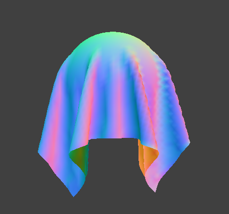
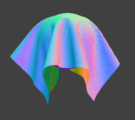
Part III: Collision Detection with Objects
Sphere Collision
In part 3 of the project we added object collision to our cloth simulation starting with sphere intersections. To implement this, we had to think about when the cloth would be hitting or intersecting with the sphere which mostly involved finding and comaring the point mass's position to the tangent point on the sphere. Once we have this tangent point, we can apply a correction vector onto the position of the point mass such that its new position will be on the surface of the sphere. As a result, we are able to simulate the effect of a cloth colliding with a sphere. Just as in previous parts, we can change the attributes of the cloth to give different affects of the simulation however in this case, they will change the way the cloth collides with the sphere.
In the following images, for example, we can see that increasing the value of ks makes the cloth firmer and therefore makes it more difficult for the cloth to bend as it hits the sphere. When ks is low at 500N/m, the cloth deforms and bends to a great extent over the sphere while the cloth with ks set to 50000 N/m does not bend as well. In fact if ks were to be increased enough, the cloth would most likely bounce off the sphere once it intersects with the surface.
 ks = 500 N/m
|
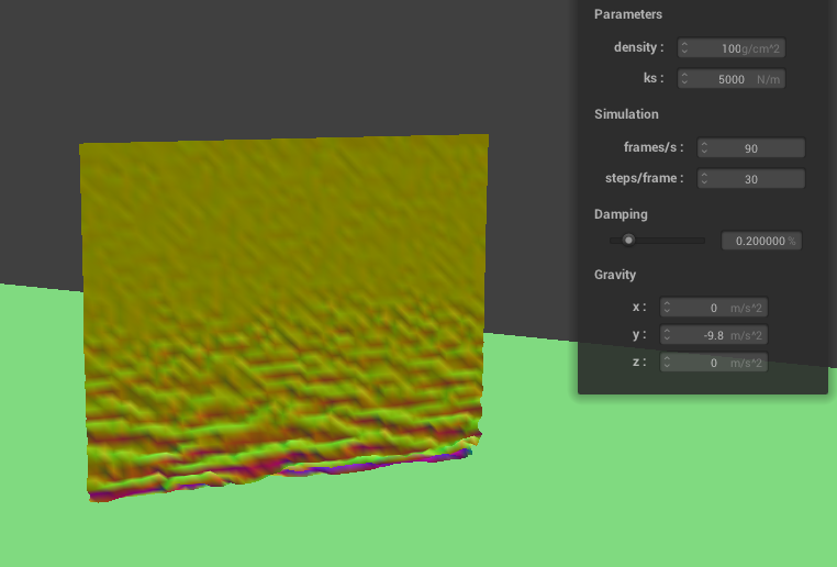
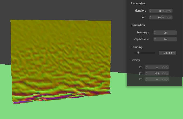
 ks = 5000 N/m
|
 ks = 50000 N/m
|
Plane Collision
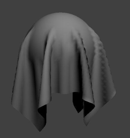
Many of the same concepts can be applied to implement plane collision with our cloth. Similar to our sphere collision, we will to identify a tangent point of the point mass to the plane surface and apply a correction vector to this point mass's position. This time we will need to make greater use of the plane's normals to identfy if we have intersected with it. After these corrections are made to the point masses, we can see our cloth sitting peacfully on the surface of the plane at the end of the simulation!
 Plane Collision in Wireframe
|
 Plane Collision with Texture
|
Part IV: Self Collisions
Though our cloth is able to successfully collide with other objects, it isn't able to collide or fall against itself the way cloth should be able to: in part of 4 of the project we implementation self collisions to fix that. Doing this required the use of a hash map structure that took unique keys or hash positions and mapped them different vectors of PointMasses. These vectors represent all of the point masses that are shared in that region of 3D space or in that key. Using this hash map we can effectively test whether a given point mass will collide with another point mass, however now we can simplfiy this calculation and only test the point masses in the current hash key rather than all of the point masses in 3D space. Once these tests for collision are made, we can see that the cloth simulation now collides with itself in a more realistic way than before when the cloth would all roll into one bundle. In the following images we can see that the cloth starts out straight, hits an initial collision with itself and continues colliding until it reaches a restful state.
 Initial Collision
|
 Self Collision Continues
|
 Restful State
|
As in other parts, we can see that changing the value of ks changes the end result of the cloth simulation. When ks is lower, for example, the cloth once again appears thinner and wrinkles much more than when ks is set at a higher value. The difference can be visibly seen in both the inital collision of the cloth as well as the restful state: in the lower ks image, the cloth ends up appearing shriveled and wrinkled into itself compared the more firm folds of image below that. In the initial collision, we can also note that the wrinkles are much more concentrated in a dense area when ks is low versus being more spread out when ks is larger.
 Lower ks Inital Collision
|
 Lower ks Restful State
|
 Higher ks Initial Collision
|
 Higher ks Restful State
|
Changing density also varies the collision of the cloth: when density is lower we can see that the folds are larger and more spread out in the intial collision and the cloth forms a more solid shape in its restful state. In comparison, when density is higher, the wrinkles become smaller and more concentrated in the initial collision and result in the cloth looking thinner in the restful state.
 Lower density Inital Collision
|
 Lower density Restful State
|
 Higher density Initial Collision
|
 Higher density Restful State
|
Part V: Shaders
In the final section of project 4, our goal was to implement various shaders in the GLSL programming language. Shaders give us the ability to simulate various effects, textures, and displacements of normals without having to wait long periods of time for detailed pathtracing renders to calculate lighting and effects in the scene. Though the final results may look slightly different compared to our work in project 3-1 and 3-2, we are still able to simulate many of the same materials we calculated previously such as diffuse & blinn phong shaders, texture mapping, bump & displacement mapping, and mirror shaders. Since my final project for this class will be based on creating a custom shader, I'm very excited to build upon the mechanics we learned from this section.
Since programming these shaders took place in a new language (GLSL), there were some things that took a while to get used to. For example, similar to C++, GLSL has two file types for each shader that are needed to make the shader fully functional: a .vert and a .frag file. The .vert file will declare many of the methods, variables, and data that is taken as an input, and passes this information along to the .frag file where the main() methods and other crucial functionalities are written. This functions somewhat similarly to C++ and its .h and .cpp files, with both pieces being very essential to the overall puzzle. Combined, we are able to create custom shaders that simulate many lighting and texturing effects based off of the same equations and logic for the work we did in project 3.
Blinn-Phong & Diffuse Shaders
The first two shaders we implemented were the diffuse shader and the blinn-phong shader. It makes a lot of sense to combine these shaders as one section of thought since the blinn-phong equation relies heavily upon diffuse shading. For example, looking at the equation we have written below, we can see that phong shaders are built upon 3 essential terms: the ambient component, the diffuse material, and the specular lighting.
L = (ka * Ia) + (kd * I/r2 max(0,n⋅l)) + (ks * I/r2 * max(0,n⋅h)^p;
ka * Ia represents our ambient componenet, (kd * I/r2 max(0,n⋅l)) represents the diffuse material, and the (ks * I/r2 * max(0,n⋅h)^p term is the basis for most of the specular effects on our final shader. Looking at the images below, we have those three terms isolated into their individual components and when combined they form the final Blinn-Phong Shader! Manipulating the values ka, kd, and ks allow us to control the ambient component, diffuse, and specular effects on the shader respectively.
 Only Ambient Component
|
 Only Diffuse
|
 Only Specular
|
 Complete Blinn-Phong Shader
|
Texture Mapping
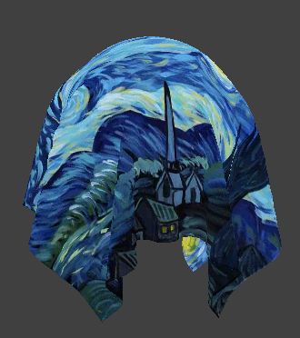
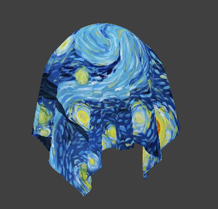
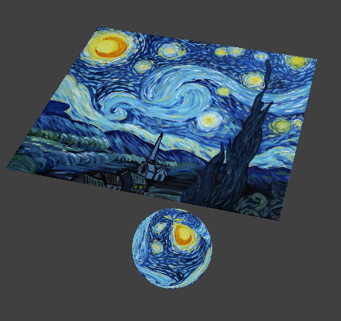
We also had the opportunity to create texture mapping effects using a custom shader. This harkens back to project 1 in which we carefully mapped u,v coordinates from a texture space onto a screen space. Here, we are similarly making us of u,v coordinates to map our texture onto our shader, and this allows for some creative uses of textures. For example, you can find a simple image online and transport our cloth into the magical world of Vincent Van Gogh's art.
A Starry Night...
Bump & Displacement Mapping
Another effect we can simulate with shaders is texture bump and displacement mapping which gives some height to the texture of our cloth. With bump mapping, we are "faking" the illusion of changing the normals on our mesh and cloth, while displacement mapping will actually alter the physical surface of the mesh. We can see the difference between the two images below in which one has the texture imprinted on the cloth while the image on the right has changed the geometry of the cloth and the sphere.
 Bump Mapping on Texture 4
|
 Displacement Mapping on Texture 4
|
We can change the coarseness, or the subdivision level, of our sphere to give slightly different effects on the simulation and the texture mapping. For example, when -a & - o are set to a lower value we can see some stretching on the bump and displacement map versus when -a & -o are set much higher. These effects are much clearer when -a & -o are set drastically low at 4 for example.
 Sphere Coarseness = 16
|
 Sphere Coarseness = 128
|
 Bump Mapping: -a -o = 16
|
 Bump Mapping: -a -o = 128
|
 Displacement Mapping: -a -o = 16
|
 Displacement Mapping: -a -o = 128
|
Mirror Shaders - Environment Mapped Reflections
Finally, we implemented mirror like effects with a shader in GLSL. This was one of the materials that we simulated back in project 3-2 and required several methods of complex code and pathtracing to achieve. However, with our Mirror Shader, we are able to recreate many of the same effects without the need for long render times and calculations. The effect is of course slightly differen than what we did in the last project, but it certainly is an efficient, cost-effective, and creative alternative for pathtracing expensive materials.
 Mirror Shader
|
 Mirror Shader
|